When developing circuits, one always has to deal with components that have tolerances that can influence the circuit's functionality to a greater or lesser extent. To determine the influence of component tolerances on the output variables of interest, a simulation with LTSpice is a good option. Common methods such as Monte Carlo analysis are already integrated into LTSpice. This article focuses on a simplified, significantly faster analysis method, worst-case analysis, which considers only the extreme limits of component tolerances.
Worst case with a simple power source

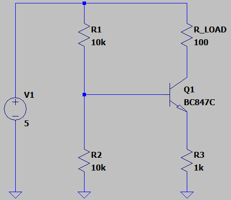
In this example you can see the construction of a simple current source with an npn transistor, 3 resistors (R1, R2 and R3) and a load resistor (R_LOAD). The current through the load resistor is “load-independent” and limited to approximately 1.84 mA set.
To determine the influence of resistance tolerances of R1, R2 and R3 on the load current by R_LOAD To determine this, LTSpice offers several ready-made functions to vary component values across multiple simulation runs.
- gauss(x), a random number with Gaussian distribution with a sigma of x
- flat(x), a random number between x and -x with normal distribution
- mc(x,y), a uniformly distributed random number between x*(1+y) and x*(1-y)
All of these functions offer an advantage when it comes to the distribution of variation. However, if, as a developer, I only want to estimate the worst-case outcome of my circuit, these analysis methods are often very time-consuming, as numerous simulation runs must be completed to ensure that the boundary values of my component tolerances are met with a high degree of probability. A different method is available here, which is easily implemented with the help of two manually added functions.
Worst-case analysis functions
This worst-case analysis procedure is implemented by inserting two functions into the schematic to be analyzed as Spice directives. These functions are:
.func wc(nom,tol,index) if(run==numruns,nom,if(binary(run,index),nom*(1+tol),nom*(1-tol)))
.func binary(run,index) floor(run/(2**index))-2*floor(run/(2**(index+1)))
If both functions are copied to the circuit diagram, the component values of R1, R2 and R3 To do this, we add the function {wc(nom,tol,index)} with the corresponding values. In our example, a value of 1% was chosen for the resistance tolerance.
For R1: {wc(10k,0.01,0)}
For R2: {wc(10k,0.01,1)}
For R3: {wc(1k,0.01,2)}
Please note that, in addition to the nominal resistance value and tolerance, each component must also be assigned a consecutive index, starting at 0. To start the simulation, we still need information about the number of iterations to be performed. With three components to be varied, the number of iterations is 2^n+1. In our case, that's 9 iterations. We communicate this to LTSpice by placing the following two Spice directives on the schematic:
.step param run 0 8 1
.param numruns=8
Simulation result
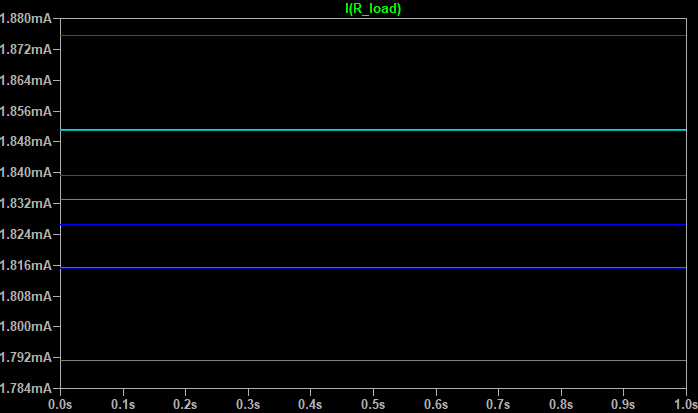
We can then start the simulation and see the following result:

Depending on which components were supplied, the current may be between 1.79 mA and 1.88 mA varies, which at a nominal current value of 1.84 mA There is already a deviation of more than 21%. This can now be interpreted by the developer accordingly, allowing an assessment of the circuit's suitability. It should also be mentioned that a more realistic assessment would also require the tolerance of the power supply and the NPN transistor, which can also be achieved with the worst-case function.
If you have any questions about this analysis method or about simulations in LTSpice in general, please don't hesitate to contact us. We'll be happy to help.


