How do I analyze electrodermal activity with Python? In this short blog post, I'll explain how you can use Python to evaluate and analyze EDA data and which libraries are useful.
1. Python for data analysis
Python is a popular programming language that provides many libraries for data analysis and processing. The library pandas used. The libraries numpy and scipy provide algorithms and functions for processing scientific and technical data.
To visualize the data and relevant results, the library can matplotlib For every step in the workflow, a tool with the appropriate functionality can be found in Python to at least simplify the work.
2. Python for EDA data
In a current MEDtech project, we are working on the processing of electrodermal activity (EDA) data. Electrodermal activity refers to changes in skin conductivity, which depend on the activity of sweat glands. In the long term, the subject's temperature and activity level have an influence.
In the short term, stress can cause a change. When conductivity varies due to stress, it is possible to observe a cluster of local maxima. For a detailed analysis of the properties of EDA data, there are several Python libraries, which I will briefly explain below.
EDA Libraries
The library pyEDA can be found on Github and offers the possibility to filter the EDA data and distinguish between phasic and tonic components. If measurements are taken over a longer period of time, the baseline value can fluctuate significantly, as described above, due to factors such as temperature.
The phasic component of the signal shows these fluctuations over time. The tonic component shows the local maxima and strives to normalize the baseline value of each maxima. The library also provides a list of all local maxima.
The same functionalities are offered by the neurokit2 This library also offers the ability to simulate an EDA signal, which is very useful for testing the rest of the Python data analysis code and its structure.
Another library for processing and analyzing physiological signals is physiology.
3. Python project structure
Generally, you should maintain a main.py script and a functions.py script. The functions.py script provides the functions. The main.py script specifies the structure and allows you to customize variables. This approach helps keep the code you work with every day short and clear.
The functions that cannot be changed are outsourced to the functions.py script. In keeping with good programming standards, these functions should be clear and testable. A test-driven development approach ensures that the functions can be clearly differentiated and must be tested individually and independently of one another.
For a project of this type, saved EDA data must be loaded. In doing so, you may need to distinguish whether you want to evaluate a single file or compare multiple files. Once you've taken a measurement, you can evaluate that measurement; later in the project, you can compare all previous measurements.
The functions.py script provides the functions needed to load the respective data in both cases and create a corresponding data structure for processing. The main.py script then simply specifies the path to the files and changes a variable to determine which mode to use.
The same principle can be used to determine whether a signal should be simulated, which data should be visualized, and how data processing should be structured. It is important to ensure that the main script is clear and that all repetitive structures are outsourced as functions.
4. Application example
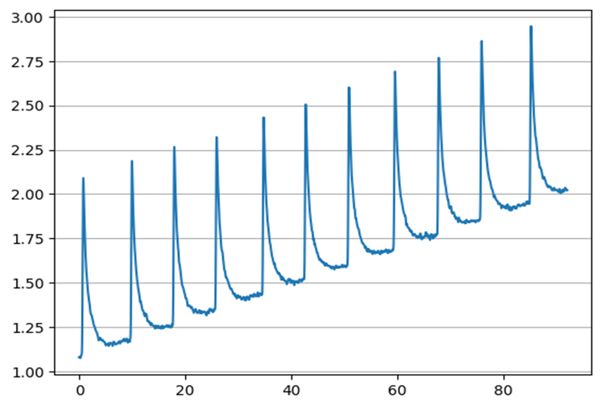
Using the neurokit2 library, an EDA signal was simulated in Figure 1. The main components of an EDA signal can be seen in this simulation. The local maxima indicate electrodermal activity. The signals usually contain drift.

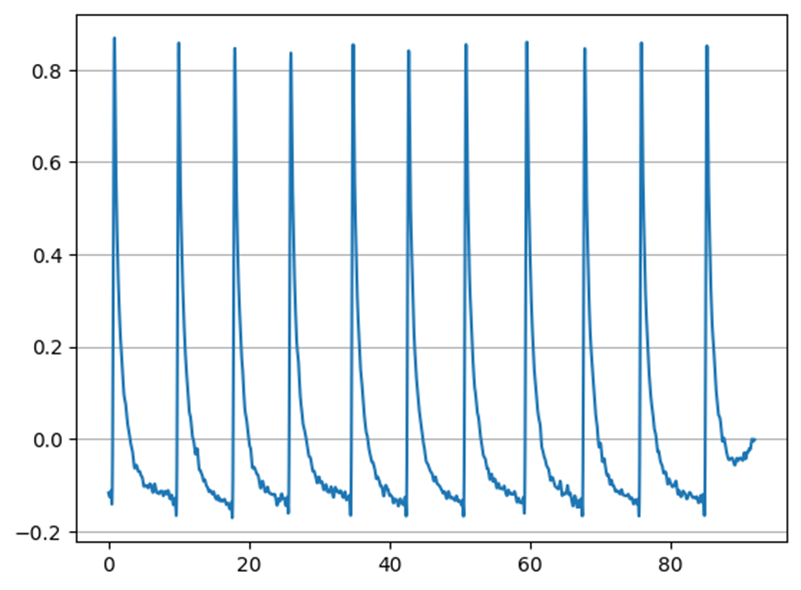
In Figure 2, the drift was removed using neurokit2 to view only the phasic component of the signal. The overall amplitude of the signal is not relevant for processing.

During processing, general information about the EDA signal is also generated, which is stored in a variable in the format shown in Figure 3.

